Now technologies allow us to create artificial materials and nanostructures which are absent in the Nature. Such nanostructures could be built on the atomic level by a precise deposition of small group atoms (atomic layers) and even isolated atoms on a specially prepared substrate. During the deposition one can combine atoms of different chemical elements, for example, to produce sandwiches from magnetic and non-magnetic atomic layers or sandwiches of a few magnetic atomic layers covered by layers of non-magnetic metals (see Fig.2.1).

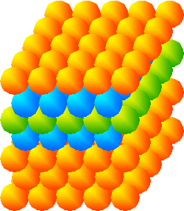
Fig. 2.1. Quasi-2D nano-sandwich constructed from the atomic layers of different chemical elements (the different elements marked in different colors).

Magnetic properties of such nanoobjects are quite unusual and puzzled. Moreover, such magnetic nanostructure, e.g. ultrathin magnetic films have a huge application potential, e.g. in magnetic memory storage and recording devices.

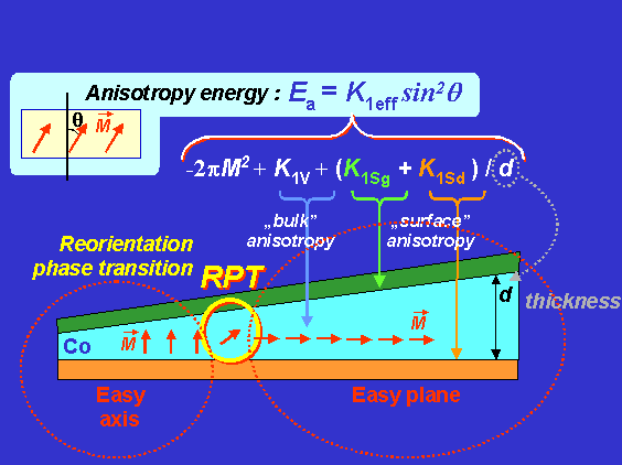
Fig. 2.2. Magnetic cobalt nanowedge (schematically). The arrows show the orientation of magnetization vector. On the left (thinner part), the magnetization state is perpendicular one, while on the right (thicker part), in-plane. The contributions from the “top” and “bottom” surfaces to magnetic anisotropy are shown.

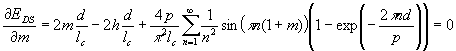
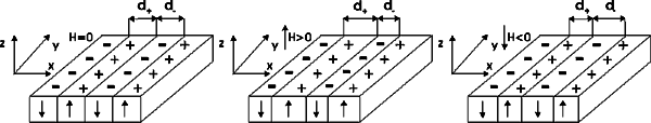
Magnetic perpendicular anisotropy of ultrathin ferromagnetic films is one of fundamental interests of magnetism of low dimensional systems (with dimensions between 2D and 3D). Magnetization states, depending on film thickness, are illustrated in Fig.2.2. For ultrathin film the anisotropy energy E_A is described in the following form .

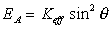
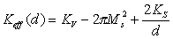
There are different sources for the anisotropy rising: crystalline (or “bulk” anisotropy), the surface anisotropy due to the broken symmetry; shape anisotropy and etc. These contributions in different ways depend on the film thickness. It is commonly assumed to describe the thickness dependence of the effective anisotropy energy of ultrahin films as

(2.1)

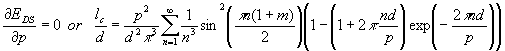
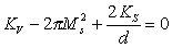
where K_V is the bulk “volume” anisotropy constant, K_s is the surface anisotropy constant. The second term in Eq.2.1 describes the demagnetization energy which is -2 Pi M_S², for film in the monodomain state. It is possible to realize vanishing of the constant K_eff (/e.g. changing the film thickness)

(2.2)

So, at d=d₁ (as K_eff (d₁ )=0). For cobalt films, depending on the grown condition, substrates and coverage, d₁ typically varies from 1.5 to 1.8 nm.

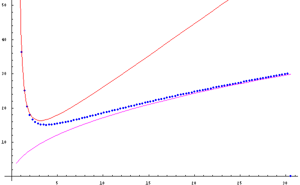
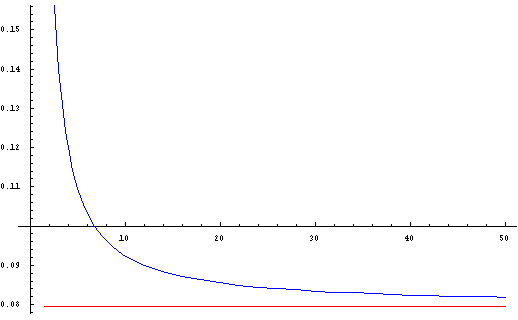
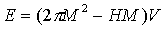
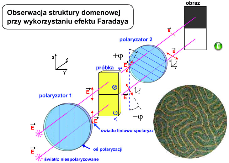
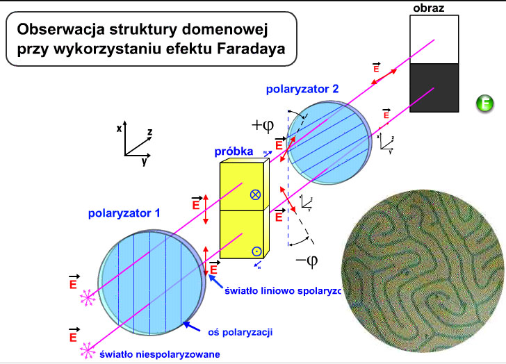
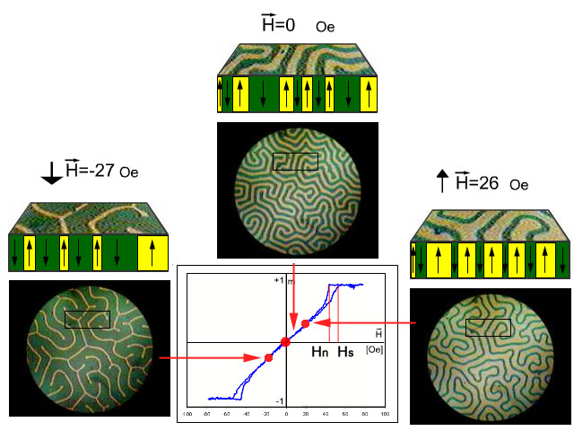
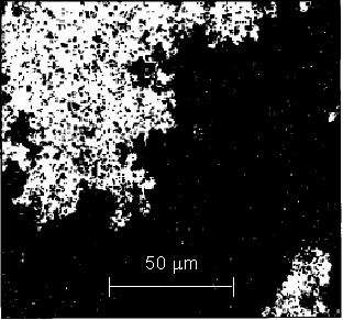
Domain structures and magnetization processes for Co in an out-off plane state (d < d₁ ) differ from those which observed in micron-sized films. Such films may exhibit a square type of hysteresis loop shown in Fig. 3.2. Domain structures could be formally described using the models from the previous chapter, see Eqs.1.14 and Eq.A2 and Eq.A3. It gives the domain period in the range from ~100 km to hundreds of nanometers as the cobalt thickness increases from d=0.8 nm to d₁ ~= 1.79 nm [1]. However, for thinner films the domain structure geometry is mainly governed by coercivity rather than magnetostatic forces. Fig. 2.3 shows the domain structure registered without magnetic field in the cobalt film with d=0.8 nm [2] (d < d₁)). One can see the domain size is much smaller than that predicted by the above theories. Such magnetic domain states are out-of-equilibrium but they are long-time living what could be very useful for applications. It is necessary to use quite different physical basis to describe domain geometry and magnetization processes – taking into account a spatial coercivity distribution one can numerically simulate domain structures in ultrahin films. The result of such simulations is shown in Fig.2.4 [2].

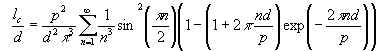
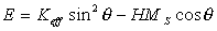
For d>d₁ the magnetization vector lies into the film plane and the film becomes in-plane magnetized. There are no magnetic domains caused by magnetostatics. It is easy to describe magnetization process for d>d₁. Let us consider a simplified case allowing the magnetization vector to coherently rotate in a homogeneously magnetized film. In this case the total film energy is given by

(2.3)

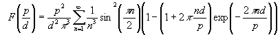
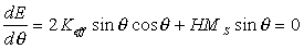
where θ is the angle between the normal to the film surface and the magnetization vector, H is the magnetic field applied along the film normal. In equilibrium the inclination of magnetization from the film normal corresponds to the minimum of the energy (Eq.2.3). So,

(2.4)

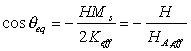
By solution of Eq.2.4 we find the equilibrium magnetization orientation, θ_e as

(2.5)

where the normalized magnetization component perpendicular to the film plane linearly depend on magnetic field normalized by the anisotropy field, H_A,eff = 2 K_eff / M_s .

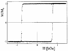
Fig. 2.3. Domain structure of ultrathin cobalt with d=0.8 nm and the magnetic hysteresis loop obtained with using the Kerr effect [2].

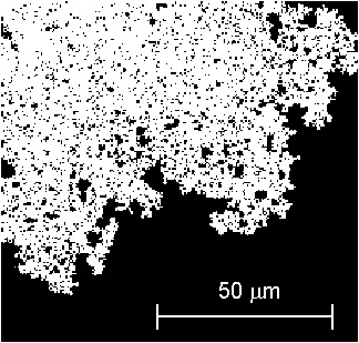
Fig. 2.4. Simulated domain structure of ultrathin cobalt with d=0.8 nm [2].

References

1. M. Kisielewski, A. Maziewski, T. Polyakova, and V. Zablotskii. Wide-scale evolution of magnetization distribution in ultrathin films. /Phys. Rev. B/ 69, 184419 (2004).
2. J. Ferr�, V. Grolier, P. Meyer, S. Lemerle, A. Maziewski, E. Stefanowicz, S. V. Tarasenko, V. V. Tarasenko, M. Kisielewski and D. Renard. Magnetization reversal processes in an ultrathin Co/Au film /Phys. Rev. B,* */55, 22, 15 092 (1997).

Now we analyze magnetization process in a film with the stripe domain structure (DS) neglecting the domain wall width, see Fig.2. The total volume energy density of DS is the sum of the domain wall, Zeeman and demagnetizing energies:

(1.8)

For periodical stripe domains with domain size D (means size of a domain magnetized opposite the applied field) the two first terms in Eq.8 can be easily obtained from a geometrical consideration. So, Eq.8 now becomes

(1.9)

with m= (D₊-D_–)/p. The demagnetizing energy is a rather complicated function and it can be represented as a series of its parameters (see the third term in Eq. A1, see the Appendix). The energy (Eq. 1.9) has two independent parameters describing domain geometry (e.g. m and p or D₊ and D_–) which can be used for E_DS minimization. We choose m and p. So, the equilibrium normalized magnetization and DS period are defined by the two equations:

(1.10)

and

(1.11)

The explicit shape of Eqs. (1.10) and (1.11) one can find in the Appendix. Here we discuss the numerical solution of the system of equations (1.10) and (1.11). They are plotted in Fig. 1.3-1.5. In Figs. 1.3 and 4 we plot the film magnetization and inverse reduced domain period (p/d) vs H/4 π M_S for different values of the ratio between the characteristic length and film thickness.

Using Eqs. 1.10,.11 one can obtain the useful, for experiment analysis, description of: (i) domain period p₀ for H/4π M _S <<1 and (ii) the initial susceptibility χ (=dM/dH _H→0). In zero-field case the domain period is determined by the magnetostatic and domain wall energies competition and the equilibrium p₀ can be easily calculated from the equation (see the Appendix):

(1.12)

where F(p₀/d) is the function defined in the Appendix and plotted Fig. 1.5.

Knowing the material film parameters l_c and d one can calculate the zero-field domain period with the help of the plot shown in Fig. 1.5, and contra versa. Solving numerically Eq.12 we find the equilibrium domain period as a function of the film thickness, see Fig. 1.6. It is important to note that the equilibrium domain period reaches its minimum at the certain film thickness which real meaning depends on the characteristic length of material. In the limiting case – large film thickness – the domain period grows proportionally to d^1/2 as it is predicted by the above simplified theory (see Eg. 1.3). The Fig. 1.6 allows us compare the results obtained by rigorous calculations (Eq. 1.12) and the simple model (Eq. 1.3).

The initial magnetic susceptibility is given by χ = dM/dH =(1/4 π ) dm/dh and can be found by differentiating of Eq.(A1) with respect to h

(1.13)

Thus, Eq. 1.13 gives the initial susceptibility of stripe domain structure as a function of domain period (see Fig. 1.7). Passing in Eq.(1.13) to the limit p₀→0 (which is a case of smallest domain wall energy and a dense domain structure, e.g. because of low anisotropy constant) one can arrive at χ₀=1/4 π. The same result was previously obtained from Eq. 1.6 on the basis a simplified model. In the opposite limit, when p→∞ (or p>>d) Eg. 1.13 gives that χ→∞. Indeed, as it seen from Fig. 1.3 the susceptibility becomes infinity large before the saturation (the jumps on the m(H)-curves). Obviously, after saturation χ=0. Notice, the right side of Eq. 1.13 only includes geometrical parameters of the film and domain structure: d and p. In general, the magnetic susceptibility is affected by many factors, e.g. coercivity. The last may be a reason for a difference between values of χ measured from the virgin magnetization curve (or magnetization hysteresis loop) and determined from a DS image. Calculations of χ from analysis of domain structure images is more easy with the help of another option our experiment – registration of magnetic hysteresis loop .

One can use these figures to determine the characteristic length and the domain wall energy of a given film. Indeed, using these plots (Figs. 1.3 -1.6) and utilizing the measured domain period and domain sizes at different values of the magnetic filed it easy to determine with the help of the above given theory the material parameters: M_S and χ

Fig. 1.3 Film magnetization (m) as a function of the normalized field (h=H /4 π MS) calculated from Eqs. A2 and A3 for different values of lc/d. Note, the curve representing the case lc/d=0 is also well described by the simplified model, see Eq. ~1.6.

Fig. 1.4 Normalized domain period (p/d) as a function of the normalized field (h) for lc/d=1/12.

Fig 1.5 Function F(p/d) used in Eq. 1.12.

Fig. 1.6. Normalized domain period (p/lc) as a function of the normalized film thickness (d/lc) for H=0. The red curve – is calculation with the Kaplan-Gehring model (Eq. 1.14), the blue one – Kooy-Enz theory (Eqs. A2 and A3), and the magenta curve is the simple dependence given by Eq. 1.3.

Fig. 1.7. Initial magnetic susceptibility as a function of the inverse domain period, z=2 π d/p. The red line shows χ=1/4 π.

Domain structures of ultrathin films.

The physics of domains in bulk materials and micron-sized films seem to be well understood. But domain patterns of ultrathin films exhibit many new features: unusually sharp thickness dependence of domain sizes and strong reconstruction of magnetization distribution in domains related to changes of magnetic anisotropy which are of great interest and essential for an understanding of fundamental physics. Now we apply the Koy-Enz theory for analysis of the thickness dependence of the domain period in a wide scale of thickness changes at H=0. Solving numerically Eqs.A5 and A6 we find the equilibrium domain period as a function of the film thickness, see Fig.6. In the ultrahin regime when d < l_ex (l_ex=(A/(2 π M_S²))^1/2, where is the exchange length and A is the exchange constant) the domain period drastically increases as the film thickness decreases. This is the case of ultrathin magnetic films (d is only a few monoatomic layers) and now such films are object of intensive studies. In the ultrathin limit the thickness dependence of the zero-field DS period can be well approximated by a simple formula (Kaplan and Gehring, 1993):

(1.14)

where b= -0.666. In the opposite limiting case- large film thickness – the domain period grows proportionally to d^1/2 as it is predicted by the above simplified theory (see Eg. 1.3).

To summarize, in Fig.6 we plot the thickness dependencies of the zero-field equilibrium domain period calculated in the frameworks of the three models: i) the rigorous Kooy and Enz model which is valid in the full scale of the thickness changes; ii) Kaplan and Gehring model (Eq. 1.13) which validity is restricted by the ultrathin regime, d <l_c and iii) a simple model (Eq. 1.3) which well describe p(d)-dependence for thicker films. As it seen from Fig. 1.6 in the ultrathin regime the domain periods could be significantly large. In general, one can expect ultrathin film in a practically monodomain state – large magnetic domains with geometry determined mainly by coercivity rather than magnetostatic forces. However, domain size drastically decreases down to a sub-micrometer scale while approaching the thickness at which the characteristic length falls practically to zero, e.g., because of decreasing the anisotropy constant.

Appendix.

The energy of a stripe domain structure is given by the Kooy and Enz model (1960):

(A1)

where m=<M>/M _S and h=H/4pM_S is the normalized field applied perpendicular to the film plane. There are two parameters which may minimize the DS energy (Eq.A1): e.g., domain period (p) and the normalized magnetization (m). The equilibrium domain structure parameters can be found by minimization of energy (A1) with respect to m=M/M_S and p, accordingly:

(A2)

(A3)

Solving Eqs. (A2) and (A3) one can calculate the equilibrium film magnetization, domain sizes and domain period as functions of the applied magnetic field. Equations A2 and A3 could be simplified if h=0 (the zero-field case). It follows from Eq.A2 that since h=0, the film magnetization m=0. By inserting the last into Eq. A3 one can arrive at

(A4)

or

( A5)

where

( A6)

References:

• C. Kittel Phys. Rev. 70 (1946) 965.
• C. Kooy and U. Enz, Phillps. Res. Repts. 15, 7 (1960).
• B. Kaplan and G.A. Gehring, J. Magn. Magn. Mater. 128, 111 (1993).
• A. Hubert and R. Schäfer, Magnetic Domains., Springer, Berlin (1998).

Now we know that magnetic domains appear to minimize the total system energy. Indeed, as usually any system try to reach the state in which its total energy becomes minimal one. The domain appearence minimizes the total energy of the sample by a lowering of the demoganetizing energy.

Let us consider the total energy of a stripe domain structure (see Fig. 1.2) of uniaxial ferromagnetic film which is infinite in lateral directions (i.e. lateral sizes L_x and L_y are much larger than d ) . In zero-field case the domains structure consists of “up” and “down”– magnetized domains and its the total energy has two contributions: the domain wall energy, E_w (which includes the anisotropy and exchange energies) and so-called magnetostatic energy, E_d:

(1.1)

The energy related with domain walls is E_w=σS N, where σ is the surface energy density of a domain wall, N=2 L_x/p is the number of domain walls in the film, S=L_yd is the area of one wall, and p is the domain period, see Fig. 1.2. So, from the above formula one can easy obtain E_w=2 σ V/p. The demagnetizing volume energy density is given by

where H_D is the local demagnetizing field which appears inside the film due to the magnetic poles on the film surfaces (see Fig. 1.1), M_s is the saturation of magnetization and H_D simple approximation by the mean value of magnetization vector M. For an infinite homogeneously magnetized film H_D=-4 πM_s and W_D=2 π M²_s. But, as it could be shown for thick enough film (d>>p), the demagnetizing field decays as Exp(-2z/p) with the distance (z) from the surface to the interior. So, the demagnetization energy of is non-zero in the layer of depth p/2 or in the volume V_dem=2L_xL_yp/2= L_xL_yp= L_xL_ydp/d=Vp/d, here the coefficient 2 appears because of the two film surfaces (magnetic poles are located on the both film surfaces: on the top and bottom ones). Notice, the demagnetizing energy is always positive and namely this increases the total system energy. To decrease the magnetostatic energy a ferromagnetic sample is divided into domains. For example, for a thick film with a stripe domain structure the magnetostatic volume energy density is less than 2 π M²_s and it can be written as W_m= η 2 π M²_s , where η is a numerical coefficient. Rigorous calculations give η=0.136 (Kittel, 1946). The demagnetizing energy of the film with the stripe domains is E_m= η 2 π M²_sV_dem= η 2 π M²_sVp/d. Finally, collecting and inserting the obtained expressions for E_w and E_d into Eq. 1.1, one can arrive at

(1.2)

Obviously, this energy has the minimum because it goes to infinity as p–>0 (too many domain walls) and as p->infty (infinite large E_d). The equilibrium domain size p₀ is found by virtue of minimization of Eq. 1.2 with respect to p:

(1.3)

where l_c=σ/ 4 π M²_s is the characteristic length which represents the key material parameter controling the domani size. In accord with Eq. 1.3 doman sizes are typically 10^-4-10^-6 cm. It follows from Eq.3 that for films of micrometer thickness the domain size grows as d^1/2. Applying an external magnetic field (H) one can change the doman sizes because of an additional contribution – the energy of interaction between the magnetic moments and the applied field (W_z=-MH , Zeeman energy). This energy should be taking into consideration in Eq. 1.2.

Fig. 1.2. Stripe domain structure of a film.

Domain structure in external magnetic field

The external magnetic field favors the domains in which the magnetization vector coincides with the field direction. In order to decrease the Zeeman energy these domains will increase their sizes while the domain magnetized in the opposite direction will be squeezed by the field. It is demonstrated in Fig. 1.2 (b and c). The film magnetization (the mean magnetic moment per unit volume) depends of the field and it is the simple relation between the volumes of “up” and “down” – magnetized domains with the size D₊ and D_–, respectively. So, it is

(1.4)

where m is the normalized film magnetization. The magnetization process is the changes of the film magnetization M(H) with the changes of the applied field. Magnetization processes are characterized by the magnetic susceptibility.

By definition the magnetic susceptibility is χ=M/H (or more precisely χ=dM/dH). In order to calculate M(H) and χ let us consider a simplified case when the domain walls have negligible small energy. In this case the total energy as the sum of demagnetizing energy and energy of the external magnetic field H

(1.5)

By virtue of minimization of Eq. 1.5 with respect to M one can obtain the normalized film magnetization as

(1.6)

Analysing the Eqs. 1.4,1.6 one can deduce : (i) when H=0 M=0 what is realised for D₊=D_–; (ii) by the definition χ=1/4π; (iii) increasing field volume of domain with magnetization along H increases and finally film is saturated (film undergoes into monodomain state) when H approaches 4 π M_S The Animation shows the magnetization process in a garnet film. More precise domain description is presented in the level 3.

Magnetic domains are areas with homogeneously distributed magnetization vector inside. The domains existence was proved by many experiments. But what is the reason for domain appearance in a sample? Domains appear to minimize the total system energy. Fig. 1 shows qualitative mechanism of the domain formation. As you know a magnetic arrow always tries to orient itself parallel to magnetic force lines (like a compass arrow in the magnetic field of the Earth). Let two magnetic arrows be parallel each other. This is an unstable configuration because the magnetic lines from the left arrow are trying to reorient the right arrow to the opposite direction. Obviously, two antiparallel magnetic arrows have less energy than those for parallel orientation. In a homogenously magnetized film the positive and negative magnetic poles (charges) distributed on the different film surfaces (top and bottom). However, similar to the two parallel oriented magnetic arrows, the given magnetic pole configuration is unstable. In such a case the system is searching ways to reach a more stable magnetic pole distribution. The example of the two arrows show us that a state with spatially remixed magnetic poles has a lower energy than the homogeneous one. This implies that in order to reach equilibrium the film should somehow redistribute its magnetic poles, for example, as it is shown in Fig.1d where several magnetic domains are shown. Thus, magnetic domains appear to decrease the sample energy associated with the magnetic charges on the film surfaces. This energy is known as the magnetostatic energy. In Fig.1 you can see the boundaries between two neighboring domains. Such a boundary has finite energy and width (typically hundreds of nanometers) and represents a domain wall – area in which the magnetization vector continuously rotates between its directions in the neighboring domains. The adding a domain wall into the film increases its total energy. The spatial period of domains is fixed by the competition between decreasing of the magnetostatic energy and increasing of so-called the domain wall energy. In zero filed case the sizes “up” and “down”-magnetized domain are the same. So, the film magnetization (the mean film magnetic moment) is zero. This is a demagnetized state of the film. Applying an external magnetic field parallel to the film normal one can change ratio between up and down-domains as well as their period. The applied filed increases the domains with the parallel magnetization orientation while the domains with the opposite magnetization are squeezed (see the Animation).. As the field increases the film magnetization grows and finally reaches the saturate state (homogenously magnetized state or monodomain state). The magnetic field strength at which the saturation reaches is named as the saturation field. In the next experimental task you can observe the domain evolution with changes of the applied magnetic field and determine by eye the saturation field.

Fig 1.1 Qualitative picture explaining mechanism domain formation (see text). There are different conventions : “+” means “N” – north magnetic pole; “-” means “S” – south magnetic pole.

Magnetic domains is a microareas ( with size normally about micrometers), with homogeneous magnetization (both in direction and amplitude) We consider magnetic layer, where magnetization vector is arranged only in perpendicular axes to the sample surface. Changebility of this case is frequently analizyse as a magnetic bar structure in infuence external magnetic fields H. Along with increase volume of this fields, domain where orientation magnetisation vector M is the same as magnetic fields H increase too. In our description we will use parameter known as reduced magnetization m, which can define based on domain structure size: m(H)=(d₊(H)-d_–(H))/(d₊(H)+d_–(H)).

Picture F1 Domain structure bar model at magnetic fields.

For investigate magnetization process and visualization domain structure we use Faraday effect (Pic. F2) – plane of linear polarizated light, after transmition by magnetic layer is rotated on angle +fi or -fi depending on magnetization vector turning in oposite directions. In accordance with the Malus law value of light after transmition by magnetic layer is proportionaly to:

Cos²(alpha +/- fi )

where alpha is a angle between main polarization plane. Turning one of polarizer can possible to turn out light transmitted by magnetic domain with defined magnetization vector, what is showing on the picture F2. Round insertion in the picture illustrate real image of magnetic structure recording by CCD camera in different polarizer position.

A	B

Picture F2 Domain structure visualization with use Farraday effect. Parts A and B respoding with two analizer – polarizer positions. (Animation – visualization of magnetic domains )

Frequently light transmitting by sample space has many domain is focusing on the single sensor then signal S(H) recoring by its can bind with the sample magnetization by equation:

S(H)=a + b*m(H)

Cooficients a i b depending on value of angles kątów alpha i fi. Measuring signal S, in various value external magnetic fields H applied to magnetic sample allow to determine magnetization (histeresis) loop for the sample m(H)

Our avaiable by Internet, experimental setup is equiped in light sensor and CCD camera (having mesh of sensors). The setup make possible for remote user measure both histeresis loop m(H) and recording pictures of domain structure in various value of magnetic field. Picture 3 illustrate magnetization process for thin magnetic layer recorded with use CCD camera and single light sensors. From its analyse we can see that incrase the amlitude of magnetic fields H increase volume of domains with the same direction of magnetization vector as a field H, increase te value m too. The sample going to monodomain state where external fields is greter then saturation field |H|>H_s. When decrase value of magnetic fields from |H|>H_s we can observe in field H_n (nucleation field) appearing domains with opposite direction of magnetization vetor to H. Value H_n its less than H_s This bahaviour is named histeresis effect. For Internet experiment we choose the sample – garnet layer, with histeresis effect in small magnetic fields (small comparing with H_n and H_s) which we can omit.

Picture F3 Example of histeresis loop and images of domain structures recorded with use our experimental setup. (Animation magnetization process). For more detailed analysis we choose rectangular area with size 20 x10 mikrometers.

With magnetic domain we can also involve very popular application in form as magnetic tapes or another magnetic media storage which its frequently use in digital/computer technology or geomagnetic earth investigate (magnetic memory of earth)

Additionaly materials we can find:

• Encyklopedia of Compentatory Physics, PWN Warszawa, 1983, Article:
  

  “Domain structure and magnetization process”, H. i R. Szymczakowie, p 585
  “Magnetooptic”, W. Wardzyński, p 590
  “Magnetic memory”, H. Lachowicz p 596

• “Physics – encyklopedical guide”, B. M. Jaworski, A. A. Dietłaf, PWN, Warszawa 1998
• “Physics”, handbook for second year of middle school, Jerzy Ginter,
• Theory decribed bar domain structure in magnetic fields.
• Magnetic hysteresis – Wikipedia
• Image processing basics

Working from any point in the World with a simple personal computer on the INTERNET, now one can obtain data from an experiment by remote control. This solution has been known in a scientific research for many years. Recently with the appearance of the new, “INTERNET” accessible laboratories for students at school/university or at home. Complicated setups a long with expensive equipment, are now connected to the most popular medium – the INTERNET. This is an excellent way to promote a Physics idea to many users who can use the experimental setup on different levels. This is a REAL EXPERIMENT !!! No simulation !!! No Java Applets !!