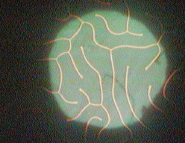
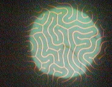
Interesting problem is describe magnetic material magnetization process, and define relationship magnetization M(H) depending on external magnetic fields H. For solving this problem we need knowledge about magnetic domain structure. We consider model based on sample with thickness h (Picture O1). The magnetization M measurred as a macro value we involve with domain structure size d₊ i d_–:

M=M_s*(d₊ -d_–)/(d₊ +d_–)=M_s*m ~~

where M_s is a magnetization of saturation which occur in single domain. On this page we can show changeability domain structure d₊(H) id_– (H) as esily as possible. On the next/linked pages we give precisly mathematic equations helpful for domain structure descriptions and software for aid this problem

Rys. O1 Struktura domenowa w polu magnetycznym H

On the start we introduce concept energy of unit sample surface E. Applying magnetic fields with force lines perpendicular to sample surface we incrase volume of domain with the same direction of manetization vector. Respecting domain structure geometry introduced on picture O1 we can easy define energy of unit sample surface in magnetic fields H E_h=-h*H*m*M_s. (Or1)

With border between light and dark domains (domain wall) is associate energy [1]. For the unit sample surface we have energy S_w. Repeated analysis geometry from picture O1 give in simple way define the energy of the domain wall (unit of surface our layer) as:

E_w=2*h*S_w/p(Or2)

For the sake of domain wall good for minimum enrgy is incrase period of magnetic structure p.

More dificult to understend (mostly in mathematics structure) is take into consideration division magnetic material onto separately, light and dark doamins. It is a result magnetostatic influence its magnetic domain parts. Each one give magnetic fields (demagnetisation fields H_d) in whole space and in neighbouring areas of sample too. This field want arrange in these areas magnetisation in antiparallel direction to domain magnetisation. Demagnetization field try to make most as possible numbers of domain, and decrace period of structure p=d₊ + d_–. Simple mathematical description for demagnetization field and demagnetization energy E_d can introduce in case ‘ideal’ magnetic layer

H_di=-4*Pi*M=-4*Pi*m*M_s (Or3a)

and demagnetization energy

E_di=2*Pi*h*m²*M_s² (OR3b)

For derive formula Or3b we use the equation Or1 where field H changing by H_d and result two times decrase (interaction parts/areas of the sample). In the sample with homogenous magnetization |H_dj|=4*Pi*M_s and demagnetization energy have the biggest as possible valueE_dj=2*Pi*h*M_s². In the case domain structure with any period demagnetization energy we can describe by formula:

E_d= 4*Pi*h*M_s² *F(h/p,m) (Or3c)

The exactly form of function F(h/p,m) is given on the next pages.

When we known magnetization of saturation M_s, domain wall energy S_w and thickness of magnetic layer h we can calculate two geometric parameters of structure: m(H) and p(H) (or d₊(H) and d_– (H)).To do this we look the minimum of complet layer energy E_t which is a sum of energy E_h + E_w + E_d=E_t. We introduce relationship beetween two “domains” parameters m and p from four quantities (three materialsM_s, S_w, h and magnetic fields H) is on the first look very complicated problem If we take the E_t form we can see that the problem can be simplify by reduced uantities. This way permit reduce problem to analyse geometric parameters of structure as a analyze function two parameters: material and reduced magnetic fields. When we divide E_t by 4*Pi*h*M_s² then:

E_tn(l/h,hg,m,h/p)=E_t/(4*Pi*h*M_s²) = 2*(l/h)*(h/p) Hg*m + F(m,h/p) (Or4e)

where parameter

• l=Sw/(4*Pi*M_s²) have a value of length and is known as a characteristic length and describe relation between domain wall energy and demagnetization energy in monodomain layer. l give also information about size of period p. Picture O4 showing relationshipp/h from l/h
• H_*=H/(4*Pi*M_s) describe relation between H and demagnetization field H_d for monodomains sample.

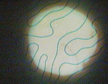
The example of relationship magnetization curve m(H_*) and the inverse domain structure period h/p(H_*)is showing on the picture O2a i O2b. From this picture we see that with incrase l/h (domain wall energy) is more easy magnetize the layer, period in domain structure is bigger too. With incrase magnetic field decrase size of structure with magnetization in opposite directions, and increase the size of domain with magnetization consistent with H and structure period. From some value of magnetic fields period is infinite and sample have homogenous magnetization (pic O2, O3)

Rys. O2a. Relationship between reduced magnetiation m=(d₊-d_–)/(d₊+d_–)) from field H_*(=H/(4*Pi*M_s)) for different value l/h parameter.

Rys. O2b. Relationship the normalized domain structure period inverse h/p from the H_*(=H/(4*Pi*M_s)) for various values of l/h.

(a)

(b)

Rys. O3. Relationship the domain width d₊ /h and d_–/h from aplitude applied magnetic fields H_*(=H/(4*Pi*M_s)). It is another presentation of results which we can see on the picture O2. Size of magnetic domain was calculated for value l/h=1/12 (a) and l/h=1/80.

Often in magnetization process describe is introduced idea of initial susceptibility chi₀=M/H . It is ratio magnetization and magnetic fields which trigger this magnetization. In case ideal layer, is easy base on formula Or4 (ehre F(m)=0.5m²) calculate chi₀i=1/4Pi. The same result we can obtain from picture 02a analyse. The picture 05 illustrate initial susceptibilityfrom h/p parametr.

Pic O4. Relationship material parameters l/h from inverse of normalized domain structure period (in null magneic fields) h/p.

Pic. O5. Relationship initial susceptibility chi₀ from material parameter l/h .

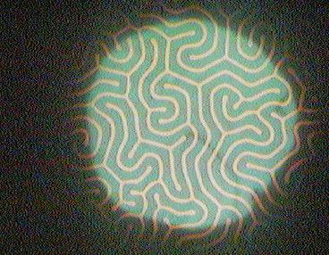
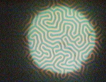
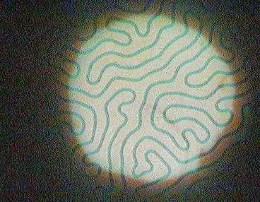
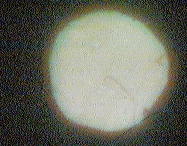
In the Internet experiment is possible, directly by picture of domain structure recording determine changebility in magnetic fields size d₊and d_– parameters in the “white” and “black” domains. It permit on determine domain structure period p and initial suscebility chi₀, more precise chi₀/M_s (because we calculate m(H)). Using this parameters in next step we can calculate materials parameters M_s and S_w. Calculate chi₀ from analyse changebility domain structure is more easy using another option our experiment – measure the histeresis loop of the sample .

Formulas and software helpful in domain changebility analyse

Calculated values w and h which can see in generated graphs dane.zip (name indicates the value of the parameter l/h)

Additional bibliography:

• Encyklopedii Fizyki Współczesnej, PWN Warszawa, 1983, Artykuły:
  

  “Struktura domenowa i procesy magnesowania”, H. i R. Szymczakowie, s 585
  “Magnetooptyka”, W. Wardzyński, s 590

Description available in digital notepad program  Mathematica or CDF ( Computable Document Format)

• symulacja-domeny-v1.cdf
• symulacja-domeny-v1.nb

CDF reader download from page : http://www.wolfram.com/cdf/

Equation and programs aided domain analysis  – Wersja HTML

Rejestracja struktur domenowych przy różnej wartości pola H. Jakościowa analiza zmienności struktur.

W naszym układzie badana próbka domenowa jest umieszczona w środku cewki podłaczonej do zasilacza którego sterowane jest możliwe poprez Internet. Pod wpływem zewnętrznego pola magnetycznego H przez nią wytwarzanym objętość domen, w których orientacja wektora magnetyzacji M jest zgodna z kierunkiem przyłożonego pola, zwiększa się.H. Efekt ten można obserwować z użyciem kamery podłaczonej do układu mikroskopowego z której zdjęcia są przesyłane do internetowego eksperymentatora wprost przez strony WWW.

Histereza probki. Niebieskimi liniami zaznaczono pole nasycenia H_n- i H_n+

Więcej na temat teorii domen magnetycznych

Wykonanie pomiaru
W celu zarejestrowania struktur magnetycznych w danym polu należy uruchomić program sterujący doświadczeniem: Obserwacja struktur domenowych w funkcji pola oraz kata skręcenia polaryzatorów . Umożliwia on nie tylko ustawianie wartości amplitudy pola magnetycznego, ale także zmianę położenia kątowego osi łatwych w układzie polaryzator/analizator (w przypadku pomiarów w funkcji H nie jest konieczna zmiana kąta nie jest konieczna). Jako wynik przesyła on grafikę w postaci wyświetlanego zdjęcia w formacie JPG. Dla osób pragnących poddać analizie obraz domeny jest przygotowana opcja umożliwiająca pobranie pliku graficznego w formacie TGA (TARGA) który przenosi dane bez utraty informacji (bitmapa). Eksperymentator powinien zarejestrować strukturę w kilku, zarówno dodatnich jak i ujemnych polach. Dobrze jest dla określenia “ciekawych pól” posłużyć się wynikiem pomiaru krzywej namagnesowania z którego można odczytać zarówno wartości pól w których próbka jest nasycona jak i posiada jescze strukturę

Wynik rejestracji struktur domenowych w różnych polach H

Pole: -6000 [A/m] – struktura całkowicie nasycona polem Hn-	Pole: -4000 [A/m]	Pole: -3000 [A/m]
Pole: -2000 [A/m] – rozrost domen typu “ciemne “	Pole: 0 [A/m] – obraz struktury w zerowym poiu	Pole: 2000 [A/m] – rozrost domen typu “jasne”
Pole: 3000 [A/m]	Pole: 4000 [A/m]	Pole: 6000 [A/m] – struktura całkowicie nasycona polem Hn+

Analiza
Po wykonaniu serii zdjęć można zauważyć na nich zmianę wyglądu struktury domenowej pod wpływem pola. Widać że wraz ze wzrostem przykładanego w danym kierunku pola następuje coraz większy rozrost jednego z typów domen kosztem drugiego. Zmieniając kierunek pola zauważamy że tendencja jest odwrotna (rozrost domen typu drugiego kosztem pierwszego).

Na podstawie tych obrazów można także odtworzyć krzywą namagnesowania. Wyliczenie i wykreślenie m(H) polega na wyliczeniu liczby piksli l_b białych i l_c czarnych: m(H)=(l(H)_b-l(H)_c)/(l(H)_b+l(H)_c) Aby to zrobić należy poddać odpowiedniej obróbce cyfrowej uzyskane obrazy domen. Po zróżnicowaniu obrazów, poprawieniu kontrastu i zbinaryzowaniu można wyliczyć wyżej przedstwione wartości funkcji m(H) dla odpowiednich obrazów domen.

General scheme of remote type of experimental set-up is shown in Fig. 4.1. Fig. 4.2 illustrates technical solution for our remote experiment “Magnetism by Internet”. In a remote experiment Internaut could : (i) change experimental conditions (in our case: amplitude of external magnetic field H; a angle between polaryzer and analyzer); (ii) choose parameters for measurements (in our case number of measurements used for signal averaging); (iii) receive measured data (in our case: voltage-signal V(H,a) from the light detector in the microscope; magnetic domain images I(H,a) from the microscope; live-image of experimental set-up – an example is shown in Fig.4.3. CGI ( Common Geteway Interface ) enables communication between www server and the computer driving the experiment. Experimental data are available for Internaut by dynamically generated www pages.

Fig 4.1 Scheme of remote experiment

Our experimental set-up is based on polarizing optical microscope with: (i) computer driven step motor changing polaryzer position; (ii) the sample – garnet film is placed in air coil producing magnetic field H perpendicular to the film plane, the computer driven power supply allows H amplitude changes; (iii) two light detectors – CCD camera and light diode.

Four types of experiment are available :

1. Study of Malus law and Faraday effect
2. Registration of magnetic hysteresis loop
3. Observation of magnetic domains
4. Observation of experimental setup on-line

The proposed experiments give opportunities to reach different levels of understanding (qualitative and quantitative) of basic magnetism. The experiments are supported by different levels of theoretical descriptions presented in chapters 1-3. Using the description an Internaut could determine different material parameters such as : Faraday rotation angle, domain wall energy, magnetization saturation,…

The goals of the following experiments are:

1. to study physics of magnetization processes;
2. to measure domain sizes and register the magnetic hysteresis loop of a thin garnet film;
3. to understand the physics of simplest domain structure – stripe domain structure, and determination of the material parameters of a given film;
4. to learn the magnetooptical domain imaging technique.

Fig. 4.1 Scheme of our remote experiment Magnetizm by Internet.

Fig 4.3 Image of experimenta set-up optical microscope with living object working aquarium with fishes.

Magnetooptical techniques are commonly used for thin and ultrathin magnetic film study. Fig. 3.1 shows results of interaction of linearly polarized light with perpendicularly magnetized film in : (i) the transmitted mode – Faraday effect; (ii) reflected mode – Kerr effect. We focus our analysis on Faraday effect application on thin magnetic films study.

Fig. 3.1. Scheme of the Faraday and Kerr effects.

Domain visualization by the Faraday effect in transmitted light mode.

Fig. 3.2 shows a scheme of the Faraday effect application for magnetic domain image formation. Unpolarized light passes through a linear polarizer, P. The polarized light is then incident on a magnetic film with two types of domains with opposite directions of magnetization, M.

Fig. 3.2. Scheme of experimental set-up for domain imaging using the Faraday effect. Parts A and B correspond to opposite angles between analyzer – polaryzer. Images of selected domain structure (in a garnet film) registered for different a are also shown. (Animation – visualization of magnetic domains )

The image formed by the transmitted light carries with it information about the domain structure of the crystal. This information is represented by intensity of the light in the final image, and the intensity is dependent on the local vector of magnetization in the crystal and the angle a between the polarizer and analyzer.

The Faraday rotation angle is φ_F and –φ_F in the two domains, respectively, see Fig.3.2. Because of the Malus law the light beams after passing the system (polarizer, magnetic film and analyzer) have different intensity which obey

(3.1)

where I₀ is intensity of the incident light. The light intensities from two domains are different:

Hysteresis loops registration using the Faraday effect

Magnetic film could be also studied using a single detector registering light passing many domains, see Fig. 3.3.

Fig. 3.3. Scheme of experimental set-up for hysteresis loops registration using the Faraday effect.

Let us consider the linearly polarized light passing through the sample with magnetization M induced by external field H. The light polarization plane rotates by the angle φ=m φ_F, where m is the normalized magnetization m=M/M_S. So the light intensity on the detector could be described by

(3.2a)

and signal measured by the detector

(3.2a)

Fig. 3.4 Magnetic field induced changes of domain structure geometry and hysteresis loop measured in the garnet film.

Fig. 3.4 shows the magnetization structure of a garnet thin in the presence of an external magnetic field. In equilibrium, without external magnetic field, the state of this uniaxial magnetic film has two oppositely oriented magnetic domains, both of which lie normal to the film plane. These domains exhibit a stripe-like labyrinthine structure. “Up” and “down” directed domain have almost the same volume at zero field H. When a magnetic field is applied in the direction of one domain magnetization, that domain becomes dominant, as can be seen in Figs. 3.4a and 3.4c.

These films with perpendicular anisotropy have been designed for use in bubble domain memories devices (a magnetic bubble is a small, stable cylindrical domain of reverse magnetization perpendicular to the surface of a thin magnetic film).